Spatial AI for Warehouse Post-Training with Cosmos Reason 1
Authors: Xiaolong Li • Chintan Shah • Tomasz Kornuta Organization: NVIDIA
| Model | Workload | Use Case |
|---|---|---|
| Cosmos Reason 1 | Post-training | Spatial AI for warehouse environments |
Overview
Supervised Fine-Tuning (SFT) is used to improve the accuracy of a pre-trained model by teaching it to follow specific instructions or understand new tasks using labeled examples. While a base model learns general patterns from large, diverse data, SFT aligns the model to specific tasks with desired outputs by showing clear input-output pairs. In this recipe, we will show how to fine-tune the Cosmos Reason 1-7B model to learn spatial intelligence tasks such as understanding distances between objects and space, the relative spatial relationship between objects, and counting.
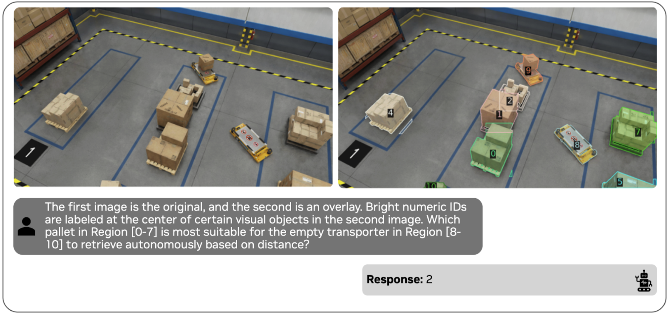
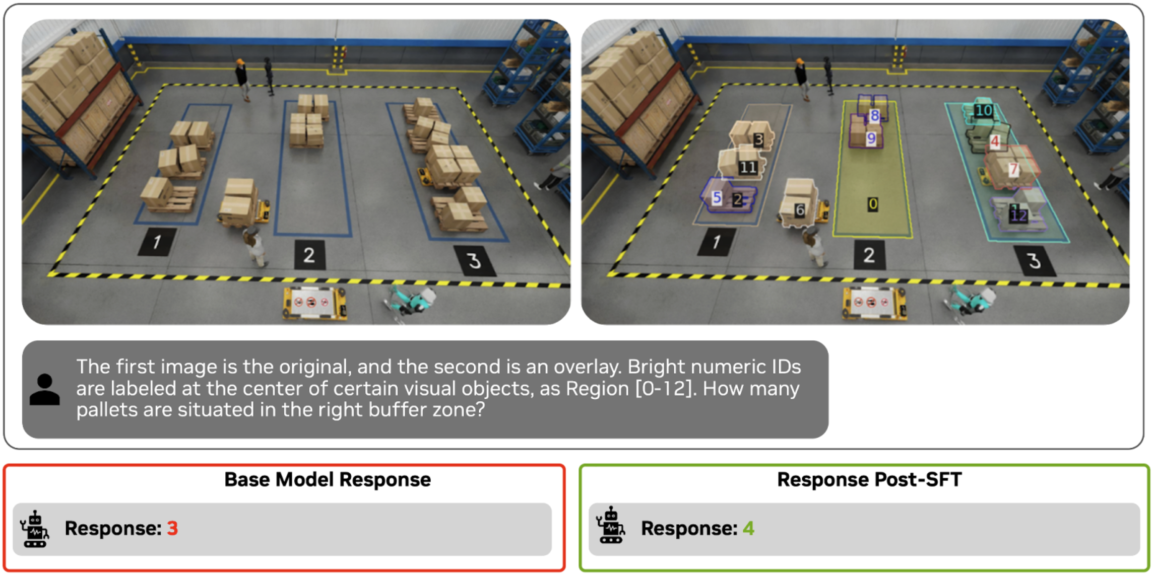
Before fine-tuning the model, let's look at the zero-shot performance of the model. Based on the question, the model has to identify the pallet closest to the transporter in region 8. Visually, the pallet identified as region 7 appears the closest to the empty transporter in region 8. Although region 2 is close, region 7 is closer. The base model incorrectly predicts region 2. Clearly there is room for the model to improve on spatial understanding tasks.
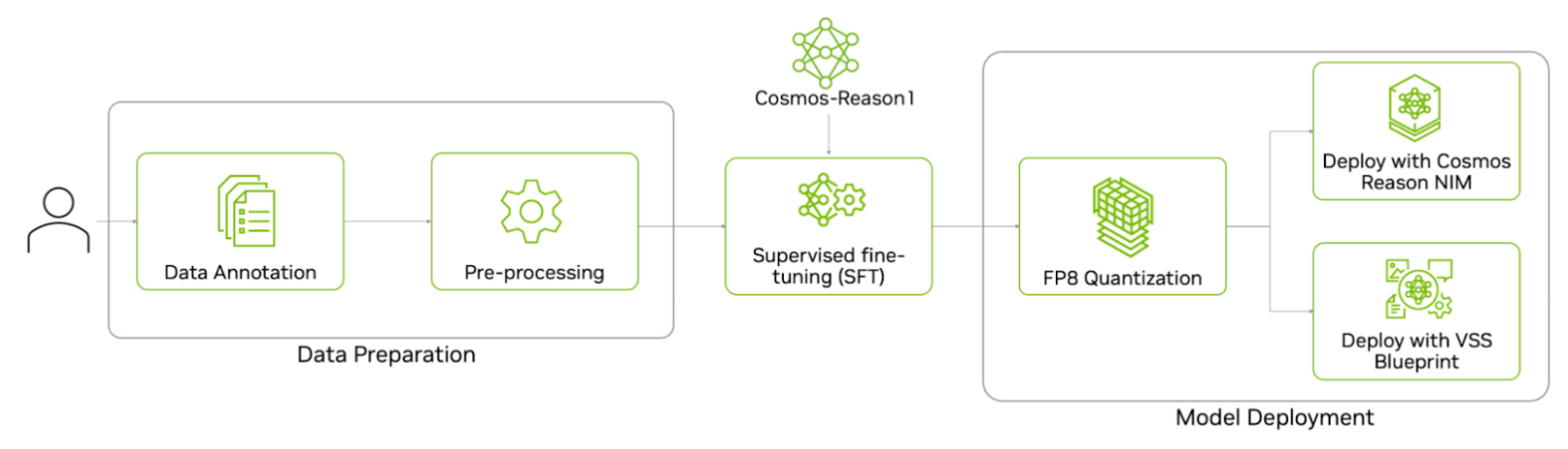
Here’s the end-to-end workflow to fine-tune the Cosmos Reason 1 model--from data preparation and supervised fine-tuning on the prepared dataset to quantizing and deploying the model for inference.
Data Preparation
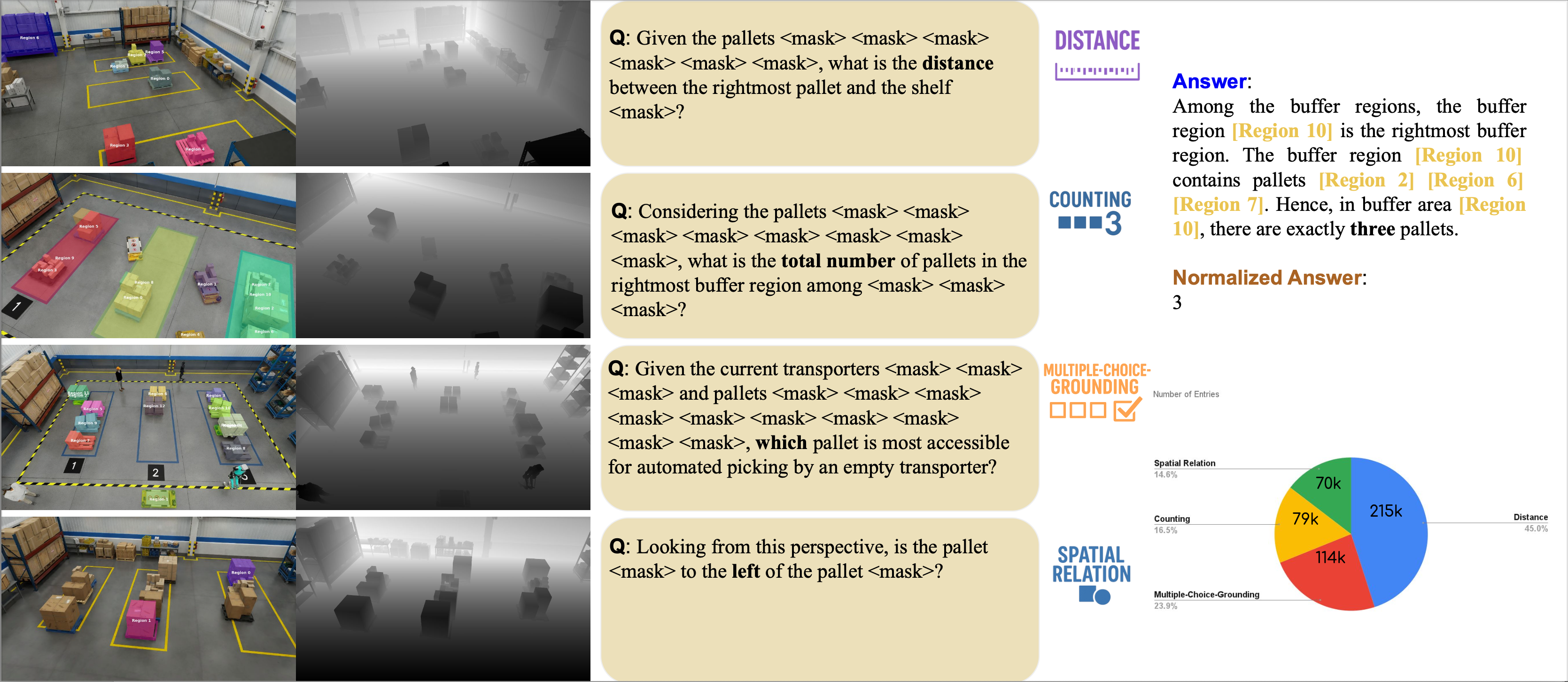
For this experiment, we will use the Physical AI Spatial Intelligence Warehouse dataset. This is a completely synthetic dataset of a warehouse with 95K images, along with around 500k annotations, which are question-answer pairs with related meta information in LLaVA format for VLM training. The tasks include distance, counting, multiple-choice grounding, and spatial relation reasoning.
The below example shows the RGB frame, depth map, annotated regions, corresponding question, and sample answers. The distribution of question types demonstrates the diversity of reasoning skills required across tasks.
Sample JSON Entry
The annotation contains several additional attributes compared to the general LLaVa format:
- normalized_answer: Quantitative evaluation with accuracy and error metrics between ground-truth and predicted answer
- freeform_answer: The original answer from 'gpt'
- rle: The corresponding masks per object in pycoco format
- category: The question category, which can be
left_right,multi_choice_question(mcq),distance, andcount
Here's an example of the annotation format:
{
    "id": "9d17ba0ab1df403db91877fe220e4658",
    "image": "000190.png",
    "conversations": [
      {
        "from": "human",
        "value": "<image>\nCould you measure the distance between the pallet <mask> and the pallet <mask>?"
      },
      {
        "from": "gpt",
        "value": "The pallet [Region 0] is 6.36 meters from the pallet [Region 1]."
      }
    ],
    "rle": [
      {
      "size": [
          1080,
          1920
      ],
      "counts": "bngl081MYQ19010ON2jMDmROa0ol01_RO2^m0`0PRODkm0o0bQOUO[n0U2N2M3N2N2N3L3N2N1N1WO_L]SO"
      },
      {
      "size": [
          1080,
          1920
      ],
      "counts": "^PmU1j1no000000000000000000001O0000000000001O0000000000001O0000000000001O0000000000"
      }
    ],
    "category": "distance",
    "normalized_answer": "6.36",
    "freeform_answer": "The pallet [Region 0] is 6.36 meters from the pallet [Region 1]."
}
Data preprocessing
For this experiment, we fine-tune the Cosmos Reason 1 model on the 80k subset of the Physical AI Spatial Intelligence Warehouse dataset. Refer to scripts/examples/reason1/spatial-ai-warehouse/ directory for more details.
Step 1: Download Data
Go to the HuggingFace Physical AI Spatial Intelligence Warehouse dataset and download the dataset.
cd scripts/examples/reason1/spatial-ai-warehouse/
hf download nvidia/PhysicalAI-Spatial-Intelligence-Warehouse --repo-type=dataset
cd PhysicalAI-Spatial-Intelligence-Warehouse
cd train/images
for file in *.tar.gz; do
    tar -xzf "$file" &
done
Step 2: Transform the VQA annotations
The complete preprocessing steps include preparing Set of Mark (SoM) image, random data sub-sampling, and conversion to the final LLaVa format. The final input to the VLM model is the original clean image, SoM image, and corresponding QA text.
Set of Mark (SoM) is a technique where you instruct the model to focus on specific “marks” in an image or text to help the VLM or LLM understand the context better and provide better responses. We will mark the object of interest with a segmentation mask and object ID. To overlay the mask and object ID on top of the original image, run the following command:
cd scripts/examples/reason1/spatial-ai-warehouse/
NUM_CHUNKS=16 NUM_WORKERS=16 python toolbox/overlay_and_save_som.py \
--original_data_root_dir /path/to/PhysicalAI-Spatial-Intelligence-Warehouse/ \
--save_root_dir /path/to/PhysicalAI-Spatial-Intelligence-Warehouse/ \
--annotation_names train

NUM_CHUNKS=16 NUM_WORKERS=16 python toolbox/overlay_and_save_som.py \
--original_data_root_dir /path/to/PhysicalAI-Spatial-Intelligence-Warehouse/ \
--save_root_dir /path/to/PhysicalAI-Spatial-Intelligence-Warehouse/ \
--annotation_names val
We will further sub-sample the dataset, and convert the results into the final LLaVa format.
python toolbox/data_preprocess.py --input_file /path/to/PhysicalAI-Spatial-Intelligence-Warehouse/train.json --output_file /path/to/PhysicalAI-Spatial-Intelligence-Warehouse/train_llava.json

python toolbox/data_preprocess.py --input_file /path/to/PhysicalAI-Spatial-Intelligence-Warehouse/val.json --output_file /path/to/PhysicalAI-Spatial-Intelligence-Warehouse/val_llava.json
Post-Training with Supervised Fine-Tuning (SFT)
After data preprocessing, convert the data into standard LlaVa format. To launch training, we follow the default cosmos-rl training command in Cosmos Reason 1 Post-Training Llava Example.
The Cosomos-Reason model uses a vision transformer that processes images in patches. The raw image starts at 1080p resolution, so we downsample the image twice to a 960x540 resolution. Since each vision token corresponds to a 28 x 28 = 784 pixel area, the result is 960/28 * 540/28 ≈ 646 tokens/frame
Hyperparameter optimization
We use the default settings in Cosmos Reason 1/sft.yaml for this SFT experiment. We changed a few of the hyperparameters to run more efficiently on 8xA100 GPUs. Since the train_batch_per_replica=32 with mini_batch=4 parameters already take care of gradient accumulation, with 8 on each single A100, the total_batch_size is 256 in our case, which largely contributes to training stability with a larger batch size. Below are the customized changes required to adapt the template config file to this post-training experiment.
Configuration Example
Here's the TOML configuration file with the key hyperparameter changes:
[policy.parallelism]
dp_shard_size=8  # for 8 GPUs for FSDP Sharding

[train]
optm_lr=1e-5     # default is 2e-6, this was better since we are adapting the model for image level training, compared to video scenarios
optm_impl = "foreach" # both 'fused' and 'foreach' should be okay,
we have 3 major categories of implementations: for-loop, foreach, and fused. 'foreach' combine parameters into a multi-tensor and run the big chunks of computation all at once, for more check https://docs.pytorch.org/docs/stable/optim.html
resume = true      # in case you want to automatically resume from any previous runs
output_dir = "/path_to_your_own_output_dir" # define your customized output_dir
enable_validation = false # turn off validation steps to save training time
master_dtype = "float32"  # you can choose use higher precision for the master weight data type for optimizers


# add config for your own dataset under [custom] attribute, we can define our own args
[custom.dataset]
annotation_path = "<PATH_TO_DATASET>/train_llava.json"
media_path = "<PATH_TO_DATASET>/"

[logging]
experiment_name = "cr1_warehouse_som_sub80k_tp1_fsdp8_node1_ep1_lr1em5"

[train.train_policy]
dataloader_num_workers = 8 # you can increase your number of data worker to load data from cpu faster
dataloader_prefetch_factor = 8 # you can increase your number of pre-fetch to save potential GPU waiting time
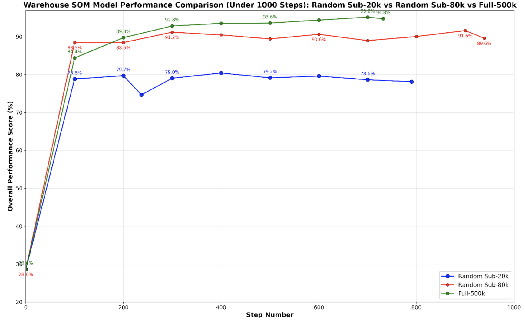
Ablation and Evaluation
We experiment with different dataset sizes (ranging from 20K to 500K question-answer pairs) and various training step configurations. For detailed analysis of our results, refer to the Results section. Below are the commands for running batch inference and generating evaluation scores.
Running Model Inference
We provide a reference script (evaluate.py) for performing parallel inference over 1K validation samples. Refer to the inference_sample.py script for updated inference code.
# Run inference with default configuration (simplified version)
python toolbox/evaluate.py \
    --annotation_path <PATH_TO_DATASET>/val_llava.json \
    --media_path <PATH_TO_DATASET> \
    --model_name <PATH_TO_MODEL_CHECKPOINT> \
    --results_dir results/spatial-ai-warehouse
Computing Evaluation Scores
To evaluate the final results and generate scores per QA category, we use the official evaluation script to compare the prediction and ground-truth:
python toolbox/score.py \
    --results_dir results/spatial-ai-warehouse \
    --official_answer_path <PATH_TO_DATASET>/val.json \
    --official_evaluation_script <PATH_TO_DATASET>/utils/compute_scores.py
Results
Qualitative Results
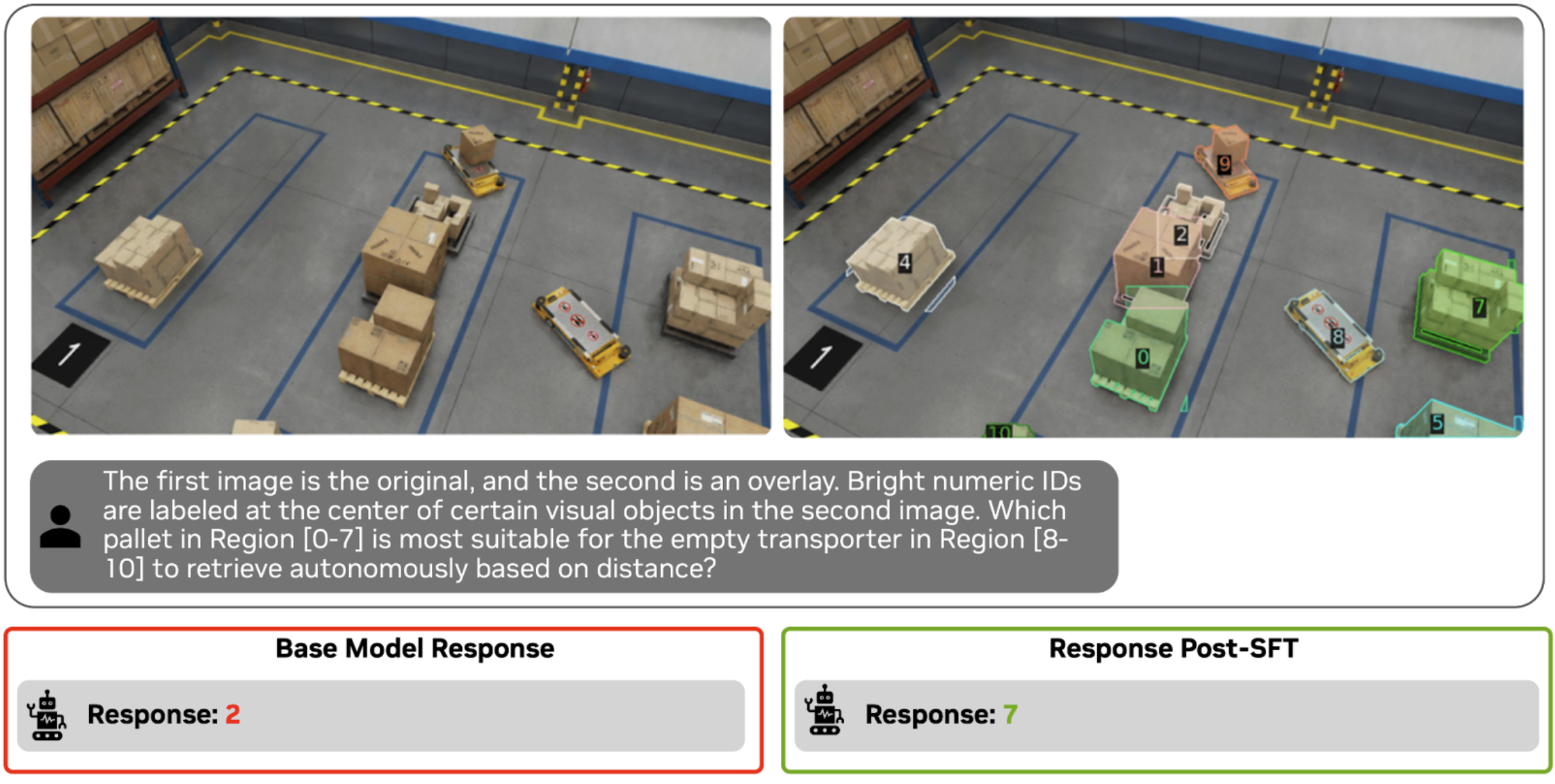
To review the qualitative improvements in the response, we prompt the same question for the base model and post-trained model. Based on the images below, you can see that the output responses have improved significantly. The post-trained model is able to understand spatial distances and count better.
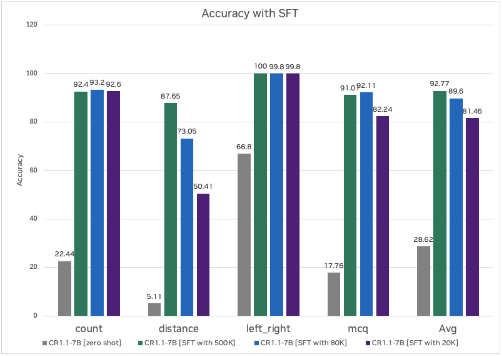
Quantitative Results
Next, let's evaluate the quantitative results for task-based accuracy for the base model versus the post-trained model. By post-training, we are able to improve accuracy significantly versus the base model. Additionally, we also experimented with different numbers of images and question-answer pairs, and, based on the experiment, we are starting to see good accuracy once we have about 80K samples. In fact, only 20K question-answer pairs are needed for "counting" and "left right" orientation tasks.
Training Time
We ran all the experiments on 1 node (8 GPUs) of A100 for three epochs. The table below captures the training time with different data sizes. The hyperparameters in the section above are for 8 GPUs; if you are using more or fewer GPUs, update the hyperparameters accordingly.
| Method | Dataset Size | Training Time (on 8 A100s) |
|---|---|---|
| SFT | 500k | 36 hours |
| SFT | 80K | 7 hours |
| SFT | 20K | 2 hours |
Model Deployment
The last step is to deploy the trained model for inference. You can deploy it using either the NVIDIA optimized NIM or through theVSS blueprint, or you can deploy it in your own application. Before deployment, we will first quantize the LLM portion of the VLM to FP8 for faster inference.
FP8 Quantization
The script to quantize the model to FP8 is provided in the NVIDIA Cosmos Reason 1 repo.
-
Clone the Cosmos Reason 1 repo.
-
Ensure you have the following dependencies to run post-training quantization (PTQ):
- Run the quantization script.
python ./scripts/quantize_fp8.py --model_id 'nvidia/Cosmos Reason 1-7B' --save_dir 'Cosmos Reason 1-7B-W8A8-FP8'
Before deploying the quantized model for inference, run evaluation on the model for accuracy and ensure quantization doesn’t introduce any accuracy regression.
Deploy on NIM
NVIDIA NIM™ provides containers to self-host GPU-accelerated inferencing microservices for pretrained and customized AI models across clouds, data centers, and RTX™ AI PCs and workstations, with industry-standard APIs for simple integration into AI applications.
To deploy a post-trained checkpoint, go to the fine-tune-model section in NIM documentation. Go to "Cosmos Reason 1-7B" tab. The NIM will automatically serve an optimized vLLM engine for this model. The model needs to be in the Huggingface checkpoint or quantized checkpoint.
export CUSTOM_WEIGHTS=/path/to/customized/reason1
docker run -it --rm --name=cosmos-reason1-7b \
    --gpus all \
    --shm-size=32GB \
    -e NIM_MODEL_NAME=$CUSTOM_WEIGHTS \
    -e NIM_SERVED_MODEL_NAME="cosmos-reason1-7b" \
    -v $CUSTOM_WEIGHTS:$CUSTOM_WEIGHTS \
    -u $(id -u) \
    -p 8000:8000 \
    $NIM_IMAGE
Deploy with NVIDIA VSS Blueprint
The VSS (Video Search and Summarization) Blueprint leverages both Vision-Language Models (VLM) and Large Language Models (LLM) to generate captions, answer questions, and summarize video content, enabling rapid search and understanding of videos on NVIDIA hardware.
By default, VSS is configured to use the base Cosmos Reason 1-7B model as the default VLM. Deployment instructions for VSS are available in the VSS documentation. VSS supports two primary deployment methods: Docker Compose and Helm charts.
For Docker Compose deployment, navigate to the Configure the VLM section under “Plug-and-Play Guide (Docker Compose Deployment)” to integrate a custom fine-tuned Cosmos Reason 1 checkpoint.
export VLM_MODEL_TO_USE=cosmos-reason1
export MODEL_PATH=</path/to/local/cosmos-reason1-checkpoint>
export MODEL_ROOT_DIR=<MODEL_ROOT_DIR_ON_HOST>
Similarly for Helm Chart deployment, navigate to the Configure the VLM section under "Plug-and-Play Guide (Helm Deployment)".
vss:
  applicationSpecs:
    vss-deployment:
      containers:
        vss:
          env:
          - name: VLM_MODEL_TO_USE
            value: cosmos-reason1
          - name: MODEL_PATH
            value: "/tmp/cosmos-reason1"
  extraPodVolumes:
  - name: local-cosmos-reason1-checkpoint
    hostPath:
      path: </path/to/local/cosmos-reason1-checkpoint>
  extraPodVolumeMounts:
  - name: local-cosmos-reason1-checkpoint
    mountPath: /tmp/cosmos-reason1
Conclusion
Supervised Fine-Tuning Cosmos Reason 1 on warehouse-specific data boosts accuracy from zero-shot levels to over 90% on spatial intelligence VQA tasks. Key insights include the following:
- Dataset scale drives causal perception: Large-scale datasets (>80K samples) provide sufficient complexity and diversity for the model to learn robust causal relationships and spatial reasoning patterns.
- Rapid convergence: Training completes within 7 hours on 80K-scale data, and it converges within the first 100 steps, demonstrating the efficiency of the fine-tuning approach.
- Seamless deployment: Workflow supports quantization and deployment via NIM or VSS for production environments.
This methodology can be applied to any physical AI domain by substituting relevant datasets, with dataset scale being a critical factor for achieving strong causal perception capabilities.
Document Information
Publication Date: October 13, 2025
Citation
If you use this recipe or reference this work, please cite it as:
@misc{cosmos_cookbook_spatial_ai_warehouse_2025,
  title={Spatial AI for Warehouse Post-Training with Cosmos Reason 1},
  author={Li, Xiaolong and Shah, Chintan and Kornuta, Tomasz},
  year={2025},
  month={October},
  howpublished={\url{https://nvidia-cosmos.github.io/cosmos-cookbook/recipes/post_training/reason1/spatial-ai-warehouse/post_training.html}},
  note={NVIDIA Cosmos Cookbook}
}
Suggested text citation:
Xiaolong Li, Chintan Shah, & Tomasz Kornuta (2025). Spatial AI for Warehouse Post-Training with Cosmos Reason 1. In NVIDIA Cosmos Cookbook. Accessible at https://nvidia-cosmos.github.io/cosmos-cookbook/recipes/post_training/reason1/spatial-ai-warehouse/post_training.html