Domain Transfer for BioTrove Moths with Cosmos Transfer 2.5
Authors: Paula Ramos, PhD Organization: Voxel51
Overview
This recipe demonstrates a complete domain-transfer pipeline for addressing data scarcity in the BioTrove moth dataset using Cosmos Transfer 2.5 and FiftyOne. It shows how to convert static images into realistic agricultural scenarios using edge-based control, Python-only inference, and FiftyOne visualization -- even when control signals (depth, segmentation) are missing.
This recipe uses FiftyOne, Voxel51’s open-source toolkit for visualizing, cleaning, and evaluating computer vision datasets. Voxel51 builds tools that help researchers and engineers better understand their data and improve model performance.
Please visit the FiftyOne Tutorial to run it all in one.
| Model | Workload | Use Case |
|---|---|---|
| Cosmos Transfer 2.5 | Inference | Domain transfer for scarce biological datasets |
Setup
Before running this recipe, complete the environment configuration: Setup and System Requirements
Motivation: Data Scarcity and Domain Gap in BioTrove Moths
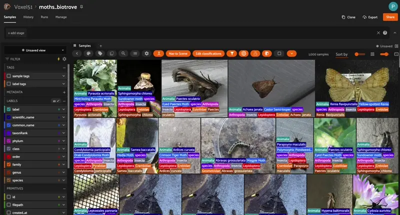
The BioTrove dataset is an extensive multimodal collection, but it contains substantial class imbalance. Moths are among the least represented categories, and most samples are collected in laboratory or artificial indoor backgrounds rather than in agricultural environments. This creates two significant challenges:
- Data scarcity — few real scenes of moths in natural field conditions
- Domain gap — models trained on lab-style images fail to generalize to outdoor agricultural settings
To build a robust classifier, we used FiftyOne’s semantic search with BioCLIP to retrieve ~1000 moth images from the full dataset. However, most retrieved samples still lacked realistic field backgrounds. The sub-dataset is in Hugging Face Hub, here.
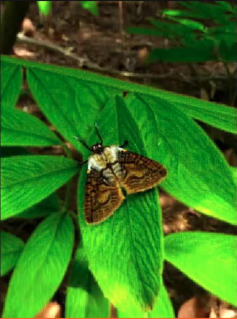
Cosmos Transfer 2.5 enables us to transform these scarce, lab-style images into photorealistic agricultural scenarios, while preserving the structure and identity of each moth. Internal experiments show 20–40% improvements in classification accuracy, thanks to better domain alignment and increased appearance diversity.
This recipe demonstrates a full, reproducible pipeline that:
- Converts moth images into videos
- Generates edge-based control videos
- Runs Cosmos Transfer 2.5 inference
- Builds a multimodal grouped dataset in FiftyOne
- Computes embeddings + similarity search
- Produces realistic agricultural moth scenes at scale
Pipeline Overview
This is the end‑to‑end flow:
- Filter and retrieve moth images using BioCLIP semantic search. Subdataset provided.
- Convert images → videos (Cosmos requires video input)
- Generate Canny edge maps as control signals
- Create JSON spec files required by Cosmos Transfer 2.5
- Run Cosmos-Transfer inference (Python-only invocation)
- Extract last frames from generated videos
- Build a grouped dataset in FiftyOne with synchronized slices
- Compute embeddings + similarity search
- Visualize results (side-by-side, embeddings, UMAP)
1. Extracting a Representative Sub-Dataset with BioCLIP
We filter BioTrove with:
- semantic search
- text queries ("moth")
- vector similarity using BioCLIP embeddings
Use:
import fiftyone as fo
import fiftyone.utils.huggingface as fouh

dataset_src = fouh.load_from_hub(
    "pjramg/moth_biotrove",
    persistent=True,
    overwrite=True,
    max_samples=1000,
)
2. Preparing Inputs: Converting Images to Videos
Cosmos Transfer 2.5 currently supports videos as inputs for inference. We convert each image into a 10-frame MP4 clip via FFmpeg.
Python version:
import os, subprocess
from pathlib import Path

videos_root = images_root.parent / "videos"
videos_root.mkdir(exist_ok=True)

for img in sorted(images_root.glob("*.jpg")):
    output = videos_root / f"{img.stem}.mp4"
    cmd = [
        "ffmpeg", "-y", "-loop", "1",
        "-i", str(img), "-t", "1",
        "-vf", "pad=ceil(iw/2)*2:ceil(ih/2)*2",
        "-c:v", "libx264", "-pix_fmt", "yuv420p",
        str(output),
    ]
    subprocess.run(cmd, check=True)
3. Generating Edge Maps (Control Signals)
Since BioTrove images lack depth/segmentation, we create Canny edge videos as control:
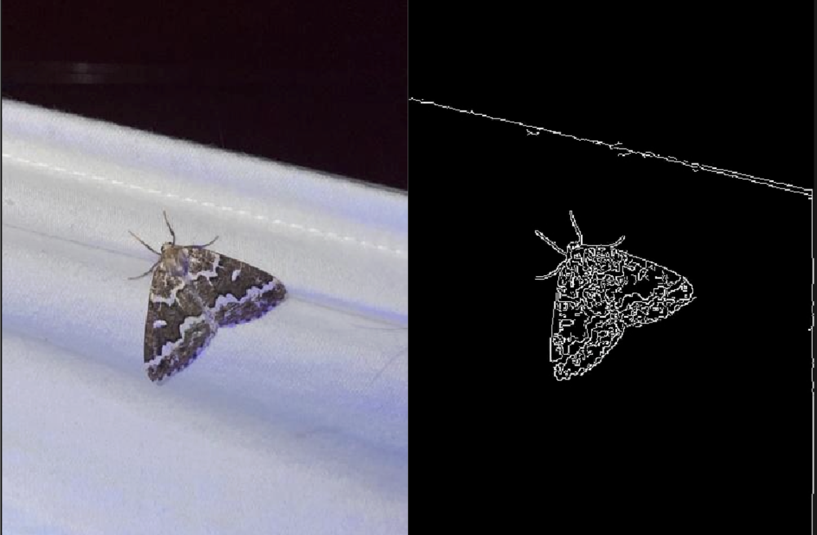
This ensures structure preservation while allowing stylistic transformation.
import cv2

def make_edge_video(input_video, output_video):
    cap = cv2.VideoCapture(str(input_video))
    fps = cap.get(cv2.CAP_PROP_FPS) or 24
    w = int(cap.get(cv2.CAP_PROP_FRAME_WIDTH))
    h = int(cap.get(cv2.CAP_PROP_FRAME_HEIGHT))

    out = cv2.VideoWriter(str(output_video),
                          cv2.VideoWriter_fourcc(*"mp4v"),
                          fps, (w,h), isColor=False)

    while True:
        ret, frame = cap.read()
        if not ret:
            break
        edges = cv2.Canny(cv2.cvtColor(frame, cv2.COLOR_BGR2GRAY), 80, 180)
        out.write(edges)

    cap.release(); out.release()
4. Building JSON Spec Files for Cosmos-Transfer
Each video needs a JSON spec describing:
- prompt
- negative prompt
- guidance
- control path
- resolution
- steps
def write_spec_json(spec_path, video_abs, edge_abs, name):
    obj = {
        "name": name,
        "prompt": MOTH_PROMPT,
        "negative_prompt": NEG_PROMPT,
        "video_path": str(video_abs),
        "guidance": GUIDANCE,
        "resolution": RESOLUTION,
        "num_steps": NUM_STEPS,
        "edge": {
            "control_weight": 1.0,
            "control_path": str(edge_abs),
        },
    }
    spec_path.write_text(json.dumps(obj, indent=2))
In this step we build one JSON spec per input video. Each spec controls:
prompt / negative_prompt – text prompts (often generated or expanded with an LLM) that describe the target domain (e.g., outdoor field imagery, natural lighting, realistic foliage, moth appearance). This is where we introduce variations in lighting, background/environment, and moth texture/appearance, while keeping the biological semantics intact.
video_path – path to the original domain video.
edge.control_path + edge.control_weight – path to the Canny edge control video and its weight, which constrains structure and motion.
guidance, resolution, num_steps – generation hyperparameters used by Cosmos Transfer 2.5.
The prompts (MOTH_PROMPT and its variations) are authored once and then expanded with an LLM to create multiple realistic variants (lighting, environment, texture), which we embed into different JSON spec files for the same base video.
To see that configuration, please review the FiftyOne Tutorial
5. Running Cosmos Transfer 2.5 Inference
Python-only invocation:
cmd = [sys.executable, str(INFER_SCRIPT), "-i", str(spec_json), "-o", str(OUT_DIR)]
subprocess.run(cmd, check=True)
After running the command, keep in mind the following parameter definitions:
INFER_SCRIPT— the path to the Cosmos Transfer 2.5 inference script you want to execute.SPEC_JSON— the path to the JSON specification file that defines the model, inputs, and control signals.OUT_DIR— the output directory where generated videos, logs, and metadata will be saved.
6. Extracting the Last Frame
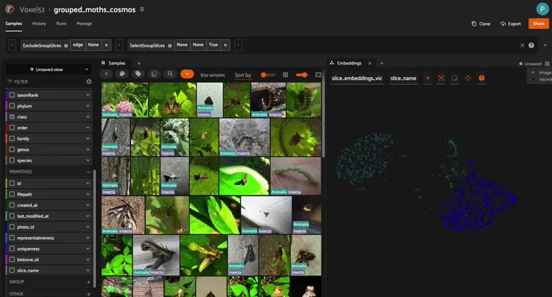
7. Building the Grouped Dataset in FiftyOne
In FiftyOne, a grouped dataset is a dataset that contains multiple slices. In the context of a grouped dataset, a slice refers to one of the components (such as an image, video, or point cloud) within each group. Each group can contain multiple slices, potentially of different modalities, which are organized under a group field. Grouped Datasets
Slices generated:
imagevideoedgeoutputoutput_last
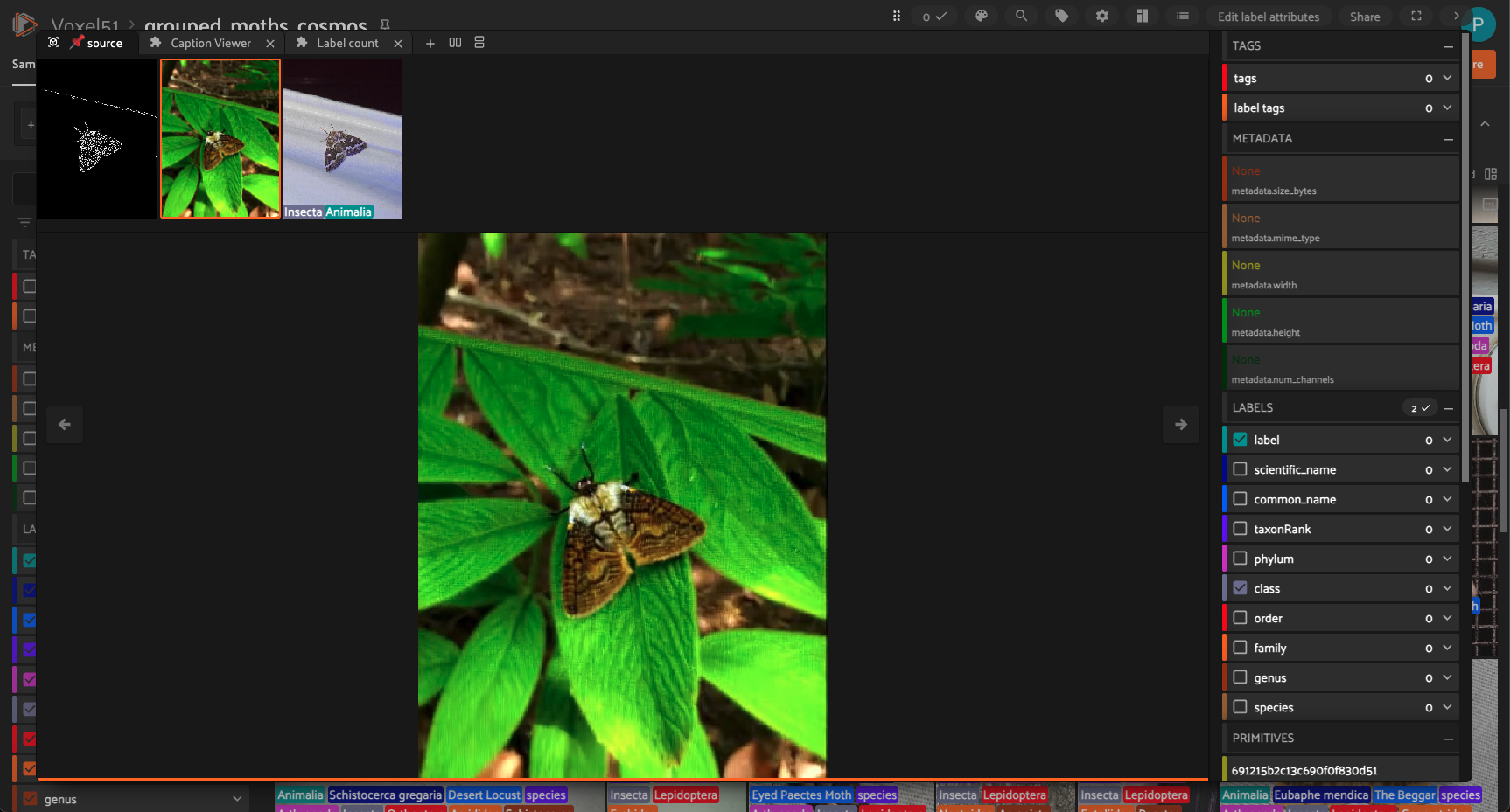
These enable synchronized side‑by‑side comparisons in the app.
8. Embeddings and Similarity Search (CLIP)
This workflow uses the CLIP model from the FiftyOne Model Zoo to generate embeddings for each sample in our dataset view (flattened_view). The embeddings are stored in the embeddings field. Then, a similarity index is created using these embeddings, enabling you to perform similarity searches—such as finding visually or semantically similar samples—within the dataset. The brain_key key_sim is used to reference this similarity index for future queries.
model = foz.load_zoo_model("clip-vit-base32-torch")
flattened_view.compute_embeddings(model, embeddings_field="embeddings")

fob.compute_similarity(
    flattened_view,
    model="clip-vit-base32-torch",
    embeddings="embeddings",
    brain_key="key_sim",
)
9. Results & Observations
While Cosmos Transfer 2.5 produced a high percentage of usable samples, the whole usability depends on refining the control signals. In particular, improving edge-control generation results in a more stable geometry and fewer artifacts in the final outputs. A promising next step is to incorporate a semantic segmentation model such as SAM3 to generate a clean moth mask. This would better preserve insect morphology and any changes in the insect shapes during the domain transfer stage.
Even with these controls, not every synthetic sample will be suitable for training. Each output should still pass a quality inspection step.
- outputs are realistic agricultural scenes
- moth morphology preserved*
- background diversity increased
- edge controls mainly maintain moth structure - we need to revisit this
- high visual coherence
morphology refers to the actual physical structure of the moth, its shape, wing outline, antennae, body proportions, and overall geometry.
Conclusion
This recipe demonstrates:
- how to address dataset scarcity
- how to create realistic domain-transfer augmentations
- how to integrate FiftyOne with Cosmos-Transfer
- how to build a reproducible Physical AI data pipeline
This approach can generalize to:
- other insect/animal datasets
- medical scarcity use cases
- robotics perception domain gaps
- any scenario lacking real-world diversity
For environment setup, see the Setup Guide. Once you have the environment ready, please use this tutorial to run everything at once. For more examples, you can explore other Cosmos-Transfer recipes in the cookbook.
Document Information
Publication Date: November 26, 2025
Citation
If you use this recipe or reference this work, please cite it as:
@misc{cosmos_cookbook_domain_transfer_for_2025,
  title={Domain Transfer for BioTrove Moths with Cosmos Transfer 2.5},
  author={Ramos, Paula},
  organization={Voxel51},
  year={2025},
  month={November},
  howpublished={\url{https://nvidia-cosmos.github.io/cosmos-cookbook/recipes/inference/transfer2_5/biotrove_augmentation/inference.html}},
  note={NVIDIA Cosmos Cookbook}
}
Suggested text citation:
Paula Ramos (2025). Domain Transfer for BioTrove Moths with Cosmos Transfer 2.5. In NVIDIA Cosmos Cookbook. Voxel51. Accessible at https://nvidia-cosmos.github.io/cosmos-cookbook/recipes/inference/transfer2_5/biotrove_augmentation/inference.html