Dataset Video Clustering with Time Series K-Means Applied to Embedding Vectors

Authors: Petr Khrapchenkov Organization: AI Robot Association (AIRoA)

Model	Workload	Use Case
Cosmos Curator	Data Curation	Video clustering by Time Series K-Means on embedding vector trajectories

Overview

This recipe shows a minimal, reproducible way to analyze and visualize precomputed embeddings (such as those produced by Cosmos Curator).

You will:

Load sample data
Interpolate data and reduce embeddings with 2D UMAP (cosine distance)
Cluster episode trajectories using TimeSeriesKMeans (softDTW) (tslearn)
Visualize the results with Matplotlib

Why trajectory clustering?

Point clustering often mixes temporal behaviors. Trajectory clustering groups entire episodes by how their embeddings evolve through time, which is often more meaningful for robotic behavior analysis and data QA.

Motivation

Many people adopt Cosmos Curator for its performance-optimized video captioning capabilities, but you can also implement advanced clustering algorithms on top of Cosmos Curator’s video clip embedding outputs. At AIRoA, we have been running Time Series K-Means on top of embeddings generated by Cosmos Curator to help categorize and cluster recordings of robot behavior during sample tasks.

Overview

This recipe demonstrates advanced clustering techniques that can be applied to the output of Cosmos Curator data curation runs. You’ll learn how to take a set of embedding vectors generated across multiple input videos, transform them into a properly formatted and structured dataset, and run a Time Series K-Means clustering algorithm to identify and distinguish similar/different input videos.

This guide focuses on a minimal demonstration workflow and provides a sample dataset and Jupyter Notebook implementation.

The Core Idea

Many people are familiar with the K-Means clustering algorithm for automatically clustering data points, but by using a distance measure appropriate for time-series (like Dynamic Time Warping (DTW), or more specifically, its differentiable variant Soft-DTW), it is possible to apply K-Means methods to entire, multidimensional time series: exactly like the data structures produced when Cosmos Curator takes a long input video, divides it into shorter clips, and then generates an embedding vector for each clip (thereby producing a "time series" of embedding vectors for each long input video).

Files

JSON sample data file
Jupyter Notebook implementation

The instructions below were tested with the following uv + jupyter notebook setup

uv init --python 3.12

uv add scikit-learn umap-learn scipy matplotlib jupyterlab tslearn

uv run jupyter lab

Recipe Steps

Understand the right data format / structures
Dimensional reduction & Interpolation
Run the Time Series K-Means algorithm
Inspect the results

Performing the analysis

1 - Input data format / structure

Once you’ve run Cosmos Curator on your target dataset, you will be able to manipulate the embedding vectors produced for each of the subdivided clips into various forms and structures which you may use for analysis. This will work better if the clips are processed with a fixed stride curator option, and that the window is fairly short. This way the embedding sequence produced by Cosmos Curator is dense enough. Five seconds is probably a reasonable starting point, but you may try decreasing the window size if your data contain higher speed movements, or increase it if the movements are slow.

For the simplicity of this demonstration, we assume you can gather the embedding vectors per clip that you are interested into a list of

# Sample of what the data structure might look like
# all_video_data = [
#  [ #all clips for video 1
#   [1.0, 2.0, 3.0,...], # embedding vector for clip1
#   [1.0, 2.0, 3.0,...], # embedding vector for clip2
#   ...
# ],
# [ #all clips for video 2
#   [1.0, 2.0, 3.0,...], # embedding vector for clip1
#   [1.0, 2.0, 3.0,...], # embedding vector for clip2
#   ...
# ]
#  ...
# ]

Note that each video may have a different number of clips, and so this cannot be a numpy ndarray going in.

To make it easier to follow the example, we’re including a sample real-world dataset from our work with robotics here, that you can download and use to follow along with our Jupyter Notebook.

import json
trajectories = json.load(open("embedding_analysis_trajectories.json", "r"))

2 - Dimensional reduction & interpolation

As-is, the data isn’t ready for Time Series K-Means yet: there are two problems we have to fix.

First, depending on the length and nature of your input videos, Cosmos Curator may have created different numbers of clips for each one. Since the Time Series K-Means we’ll be using expects the input time series to be the same length, we need to interpolate the embedding vector time series we have for each video to a common, fixed length for all videos.

Second, since our embedding vectors are living in a high dimensional space, for computational efficiency, we should perform a dimensional reduction before running the Time Series K-Means.

The interpolation function

import numpy as np

def subdivide_trajectory(trajectory: np.ndarray, n_points: int) -> np.ndarray:
    traj = np.asarray(trajectory, dtype=float)
    t_len, n_features = traj.shape
    if t_len == 1:
        return np.repeat(traj, repeats=n_points, axis=0)

    x_old = np.linspace(0.0, 1.0, t_len)
    x_new = np.linspace(0.0, 1.0, int(n_points))

    out = np.empty((int(n_points), n_features), dtype=float)
    for feat_idx in range(n_features):
        out[:, feat_idx] = np.interp(x_new, x_old, traj[:, feat_idx])
    return out

interpolated_trajectories = np.asarray(
    [subdivide_trajectory(np.asarray(traj), 6) for traj in trajectories]
)

Dimensional reduction

n_traj, t_len, dim = interpolated_trajectories.shape
flat = interpolated_trajectories.reshape(n_traj * t_len, dim)

from umap import UMAP
RUN_SEED = 353550416
flat_2d = UMAP(
    n_components=2,
    random_state=RUN_SEED,
    n_neighbors=15,
    min_dist=0.1,
    metric="cosine",
).fit_transform(flat)

3 - Run the Time Series K-Means algorithm

Now that our data is ready to go, we’ll run the Time Series K-Means algorithm from tslearn using the Soft-DTW metric mentioned above.

from tslearn.clustering import TimeSeriesKMeans

trajectories_2d = flat_2d.reshape(n_traj, t_len, 2)

RUN_SEED = 353550416
model = TimeSeriesKMeans(
    n_clusters=3,
    metric="softdtw",
    max_iter=50,
    random_state=RUN_SEED,
    verbose=False,
)
traj_labels = model.fit_predict(trajectories_2d)
centers = np.asarray(model.cluster_centers_)

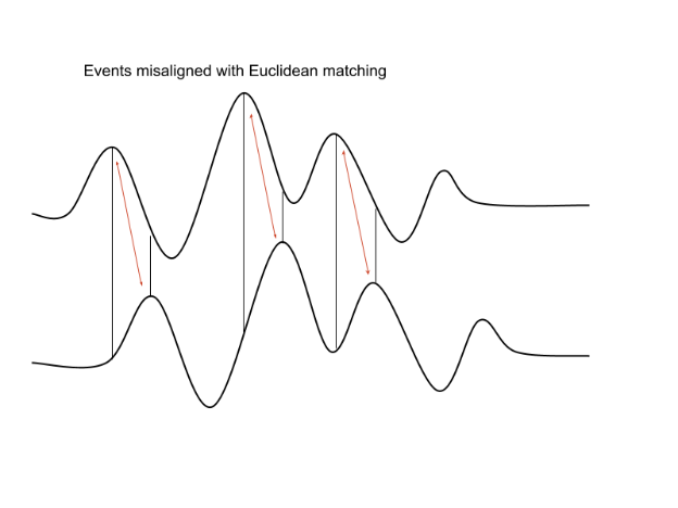
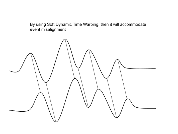
Why do we use Soft-DTW?

The primary challenge when applying K-Means techniques to time series data is choosing a suitable distance metric.

Pointwise Euclidean distances between timeseries can fail if the two time series are shifted or distorted with respect to each other on the time-axis. > Dynamic Time Warping (DTW) was developed to resolve this.

Soft-DTW is a differentiable variant of regular Dynamic Time Warping.

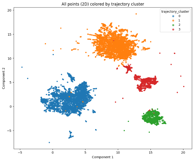
4 - Inspect the results

Finally, let’s check the results. First, we’ll visualize our clusters with matplotlib:

import matplotlib.pyplot as plt

flat_points = trajectories_2d.reshape(-1, 2)
flat_labels = np.repeat(traj_labels, t_len)

cmap = plt.get_cmap("tab10")
unique = sorted({int(x) for x in np.asarray(flat_labels).tolist()})
color_map = {cid: cmap(i % cmap.N) for i, cid in enumerate(unique)}

plt.figure(figsize=(10, 8))
for cid in sorted(color_map.keys()):
    m = flat_labels == cid
    plt.scatter(flat_points[m, 0], flat_points[m, 1], s=6, alpha=0.7, color=color_map[cid], label=str(cid))
plt.title("All points (2D) colored by trajectory cluster")
plt.xlabel("Component 1")
plt.ylabel("Component 2")
plt.legend(title="trajectory_cluster", loc="best", markerscale=2, fontsize=9)
plt.show()

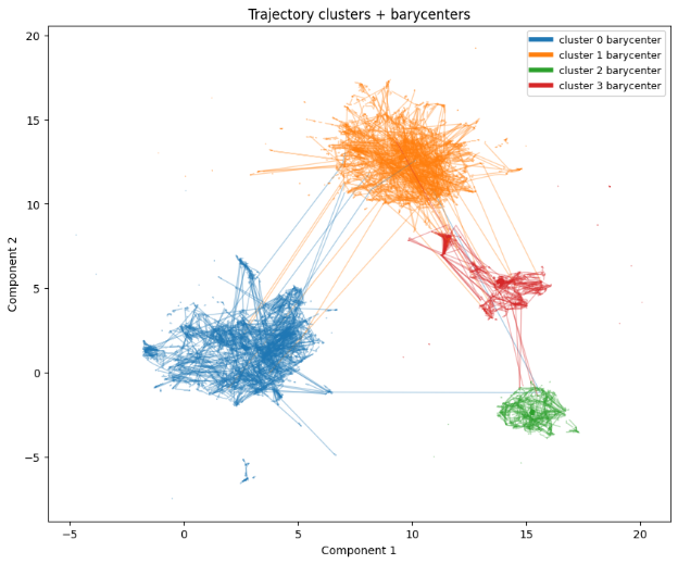
# Plot 2: trajectories + barycenters
plt.figure(figsize=(10, 8))
for i in range(n_traj):
    cid = int(traj_labels[i])
    plt.plot(trajectories_2d[i, :, 0], trajectories_2d[i, :, 1], linewidth=1.0, alpha=0.35, color=color_map.get(cid, (0,0,0,0.35)))
for cid in range(centers.shape[0]):
    plt.plot(centers[cid, :, 0], centers[cid, :, 1], linewidth=4.0, alpha=1.0, color=color_map.get(int(cid), (0,0,0,1.0)), label=f"cluster {cid} barycenter")
plt.title("Trajectory clusters + barycenters")
plt.xlabel("Component 1")
plt.ylabel("Component 2")
plt.legend(loc="best", fontsize=9)
plt.show()

Then, if you want a quantitative metric for the quality of your resulting clustering, a variety of methods are available, like silhouette scores (scikit-learn implementation) or Davie-Bouldin scores (scikit-learn implementation) to help you evaluate your performance and choose hyperparameters (like the number of clusters to use).

from sklearn.metrics import silhouette_score, davies_bouldin_score

traj_means = trajectories_2d.mean(axis=1)  # (n_traj, 2)

print("silhouette_score:", float(silhouette_score(traj_means, traj_labels)))
print("davies_bouldin_score:", float(davies_bouldin_score(traj_means, traj_labels)))

Example silhouette and Davies-Bouldin score:

silhouette_score: 0.6653785109519958
davies_bouldin_score: 0.42510679230192855