Generate Photorealistic agricultural images for robot perception training

Authors: Usman Khan • Yuri Brigance Organization: Aigen

Overview

Model	Workload	Use Case
Cosmos Transfer 2.5	Post-training + Inference	Generating photorealistic synthetic agricultural imagery for robot perception training

Soybean Transfer

Training robust perception models for agricultural robotics requires diverse, high-quality labeled data spanning crops, growth stages, weather conditions, and disease states. Agriculture presents a particularly challenging long-tail distribution problem — the number of variations across plant species, environmental conditions, and field states is enormous, and real-world data collection is slow, seasonal, and expensive.

This recipe demonstrates how to post-train Cosmos Transfer (depth-conditioned) on agricultural fleet video to generate photorealistic synthetic training images for downstream robot perception. Key result: autonomous field weeding achieved using a perception model trained with only 1% real data, with the remainder generated synthetically using this pipeline.

Cosmos Transfer is well suited to this domain because it enforces spatiotemporal structure, allowing visual variation while preserving the spatial relationships critical for centimeter-level precision agriculture. Post-training bridges the domain gap between the foundation model's visual priors and the appearance of row-crop fields — even a modest training run yields strong results on in-distribution crops and promising generalization to unseen ones.

Setup and System Requirements

Follow the Setup guide for general environment setup instructions, including installing dependencies.

Hardware:

8× A100 GPUs (e.g., AWS p4de.24xlarge)

Software Dependencies:

Cosmos Transfer 2.5 model weights and training framework
Depth estimation pipeline (synchronized RGB+D from fleet cameras, or an off-the-shelf monocular depth model such as DepthAnything V2)

Motivation: The Agricultural Sim2Real Gap

Agricultural robotics operates in one of the most visually diverse and uncontrolled environments in physical AI. A single soybean field changes dramatically across a growing season — from bare soil to canopy closure — and conditions shift with weather, time of day, weed pressure, and disease. Collecting and labeling real data across this full combinatorial space is prohibitively expensive, and much of it is only available during narrow seasonal windows.

Synthetic data generation offers a path forward, but generic world models lack the domain-specific realism needed for precision agriculture. Leaf textures, soil appearance, shadow patterns from row-crop geometry, and the visual signatures of disease are all details that matter for downstream perception.

Post-training Cosmos Transfer on fleet-captured agricultural video closes this domain gap.

┌─────────────────────────────────────────────────────────────────┐
│               AGRICULTURAL DOMAIN GAP                           │
│                                                                 │
│  Foundation model priors         Agricultural reality           │
│  ┌──────────────────────┐        ┌──────────────────────┐       │
│  │  Generic scenes      │        │  Row-crop fields     │       │
│  │  Controlled lighting │   ──►  │  Variable sunlight   │       │
│  │  Common objects      │  ???   │  Leaf morphology     │       │
│  │  Limited seasons     │        │  Disease symptoms    │       │
│  └──────────────────────┘        └──────────────────────┘       │
│                                                                 │
│  Post-training on ~3,000 fleet clips bridges this gap.          │
│  Result: 1% real data sufficient for production weeding.        │
└─────────────────────────────────────────────────────────────────┘

Zero-Shot Evaluation

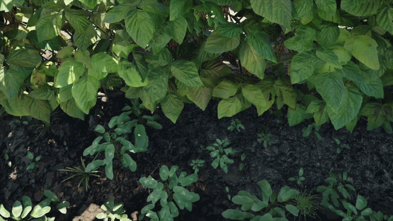
The base Cosmos Transfer 2.5 checkpoint does not perform well on agricultural data. Model outputs fail to adhere to control signals and are unable to produce photrealistic visual features, such as leaf shape and color, lighting, and scene textures.

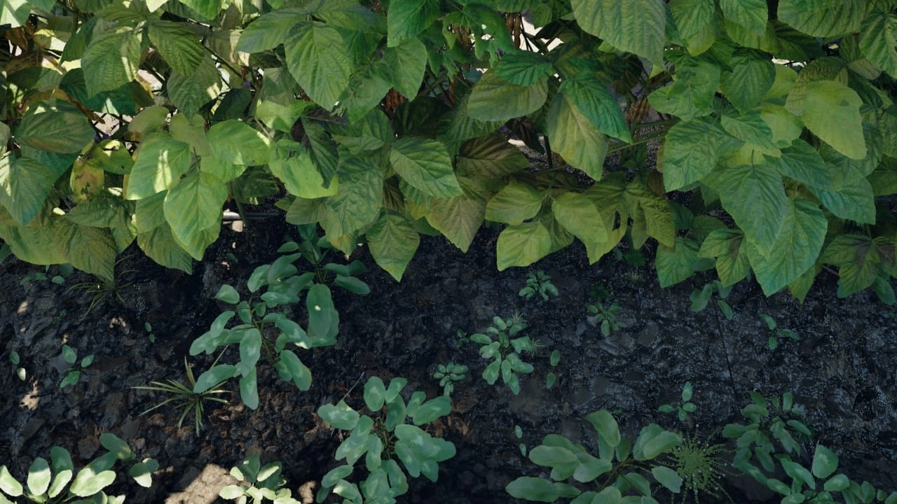3D Render

Depth Control Signal

Data Preparation

Source Data

The training data for this recipe consists of fleet-captured video clips (RGB + depth) collected across row-crop agriculture fields. The dataset includes approximately 3,000 clips of roughly 10 seconds each, covering soybean, cotton, and tomato fields with varying weed density, growth stages, and lighting conditions.

Property	Value
Source	Fleet-captured RGB+D video
Clips	~3,000
Duration	~10 seconds per clip
Original resolution	720p
Training resolution	480p
Frame rate	10 FPS
Crops	Soybean, cotton, tomato
Depth	Synchronized per-frame from fleet cameras

Depth Map Extraction

Depth maps serve as the control signal for Cosmos Transfer. This recipe uses synchronized depth from fleet cameras, but monocular depth estimation can substitute when hardware depth is unavailable.

# Monocular depth with DepthAnything V2 (when fleet depth unavailable)
from transformers import pipeline as hf_pipeline
import numpy as np
import cv2

estimator = hf_pipeline(
    "depth-estimation",
    model="depth-anything/Depth-Anything-V2-Base-hf",
    device="cuda"
)

result = estimator(pil_frame)
depth_np = np.array(result["depth"])

# Normalize to [0, 255] — 0=near, 255=far
depth_u8 = cv2.normalize(depth_np, None, 0, 255, cv2.NORM_MINMAX).astype("uint8")

Critical: Normalize depth distributions to match the conventions present in the Cosmos Transfer training data. If your inference-time depth maps use a different normalization than training, outputs will degrade. Apply the same normalization pipeline consistently across training and inference.

Dataset Formatting

Dataset Schema

Required sample components

Field	Type	Required	Description
`sample_id`	string	Yes	Unique identifier shared across RGB video, depth video, and caption JSON
`video_path`	string	Yes	Path to the RGB clip used as the primary visual input
`depth_path`	string	Yes	Path to the depth-control clip aligned frame-by-frame with the RGB clip
`crop_type`	string	Recommended	Crop class, for example `soybean`, `cotton`, or `tomato`
`field_state`	string	Recommended	Field condition descriptor, such as weed density, canopy stage, or soil exposure
`camera_view`	string	Recommended	Camera angle or mounting context, for example `angled_row_view` or `front_nav`
`weather`	string	Optional	Weather metadata if available from field logs

Recommended manifest

In addition to the folder structure below, consider including a top-level manifest such asdataset_root/clip_index.json with one JSON object per clip. This makes it easier to validate the dataset, generate captions programmatically, and subset by crop type or field condition.

Organize clips into the directory structure expected by the Cosmos Transfer training pipeline:

dataset_root/
├── videos/             # 480p, 10 FPS, clips trimmed to ×93 frames
│   ├── clip_001.mp4
│   └── clip_002.mp4
├── depth/      # Per-clip depth video, same dims and frame count
│   ├── clip_001.mp4
│   └── clip_002.mp4
└── captions/           # One JSON per clip
    ├── clip_001.json   # {"prompt": "...", "negative_prompt": "..."}
    └── clip_002.json

Latent frames: The number of latent frames (model config parameter state_t) is reduced to 16 (from the default 24) because agricultural scenes exhibit low temporal variability — crops and soil don't move significantly frame to frame, so fewer latent frames are sufficient to capture the relevant dynamics. Accordingly, num_frames is set to 61 to match.

Caption Generation

Captions are generated using a template populated with metadata from the data capture pipeline (crop type, camera angle, field conditions) and augmented with a VLM for natural language descriptions. Weather data can be appended when available.

# Caption template
CAPTION_TEMPLATE = (
    "{camera_angle} view from an agricultural robot in a {crop} field. "
    "{field_state}. "
    "{vlm_description}"
)

# Example output
caption = {
    "prompt": (
        "A field view of soybean plants growing in rows under bright direct sunlight. "
        "Dense weed growth visible between crop rows. "
        "An angled view showing green oval-shaped leaves on slender stems in dry brown soil, "
        "with strong sunlight and clear shadows."
    ),
    "negative_prompt": "blurry, overexposed, motion blur, synthetic render"
}

VLM backend: Gemini 2.5 Flash is used for natural language description generation.

Post-Training Configuration

Control Modality: Depth over Edge

Both depth and edge control modalities were evaluated for this domain. Depth control produced significantly better results. Edge control post-training showed only slight improvement over the base model.

The explanation is rooted in outdoor agricultural lighting conditions:

Condition	Effect on Edge Maps	Effect on Depth Maps
Strong direct sunlight	Shadow boundaries create spurious edges	No effect — depth is illumination-invariant
Auto-exposure variation	Causes frame-to-frame edge inconsistency	No effect
Overcast diffuse light	Suppresses real edges; gradient ambiguity	No effect
Specular highlights (wet leaves)	False positive edges	No effect

Recommendation: For any outdoor physical AI domain with uncontrolled lighting, depth is the preferred control modality over edge.

Experiment Configuration

experiment = dict(
    dataloader_train=dict(
        dataset=dict(
            control_type="depth",          # depth control for outdoor scenes
            resolution="480p",
            num_video_frames=61
        )
    ),
    model=dict(
      config=dict(
        resolution="480p",
        state_t=16
      )
    ),
    trainer=dict(
        max_iter=4000,
        save_iter=500,
    ),
    # Use defaults for other fields and/or set as appropriate
)

Key Hyperparameters

Parameter	Value	Rationale
Control type	`depth`	Robust to outdoor lighting variation
Training iterations	4,000	Loss plateaus early but quality continues improving — train longer
Resolution	480p	Sufficient for downstream weed detection pipeline
Latent frames	16	Agricultural scenes have low temporal variability
Depth guidance scale	0.8 (inference)	Strong structural adherence with room for surface detail

Training insight: Training for longer improves generation quality in ways more visible in output samples than in the loss metric. Recommend visual inspection of generated outputs at checkpoints rather than stopping at loss plateau.

Launch Training

export NUM_GPUS=8
export DATA_DIR=/path/to/dataset

IMAGINAIRE_OUTPUT_ROOT=/large/storage \
torchrun --nproc_per_node=$NUM_GPUS --master_port=12341 \
  -m scripts.train \
  --config=cosmos_transfer2/singleview_config.py \
  -- experiment=transfer2_singleview_posttrain_depth_aigen
  dataloader_train.dataset.dataset_dir=$DATA_DIR 'dataloader_train.sampler.dataset=${dataloader_train.dataset}'

Convert Checkpoint

# After training, convert DCP format → PyTorch for inference
python scripts/convert_distcp_to_pt.py \
  ${CKPT_DIR}/model \
  ${CKPT_DIR}

# Use checkpoint_ema_bfloat16.pt for all inference runs

Inference

Generating Synthetic Images

At inference time, construct prompts describing the target scene: crop type, growth stage, field conditions, lighting, and optionally disease symptoms. Prompt precision matters — specific descriptions of visual features produce better results than vague ones.

Depth guidance scale: Use 0.8. This provides strong structural adherence to the depth control signal while leaving freedom for realistic surface detail and lighting.

Depth distribution matching: Inference-time depth maps must use the same normalization as training. Mismatched normalization degrades output quality — apply the same preprocessing pipeline.

Note on single-image input: If you want to transform a single image rather than a video clip, you can loop the image into a video of the appropriate length for inference. However, note that this is an inference-only workaround — results will be lower quality than video-to-video generation because the model receives no temporal motion information.

# Inference with post-trained checkpoint
python examples/inference.py \
  --params_file agriculture_spec.json \
  --checkpoint_path ${CKPT_DIR}/checkpoint_ema_bfloat16.pt \
  -o outputs/validation/

Minimal Quickstart

Download sample dataset from Hugging Face here

Example Prompts

Healthy soybean rows, bright sunlight:

"An angled view of soybean plants growing in rows on a farm field on a bright sunny day. Green oval-shaped soybean leaves on slender stems in dry brown soil, with strong sunlight and clear shadows. Scattered weeds between the rows."

Healthy soybean rows, bright sunlight

Diseased soybeans — yellowing and wilting:

"An angled view of large soybean plants growing in a row on a farm, with scattered weeds. The crop shows signs of disease with yellowing leaves, brown spots, and wilting foliage."

Diseased soybeans

Results

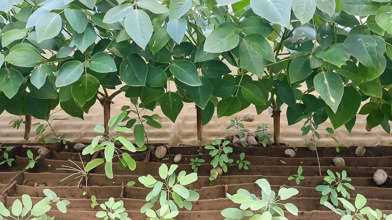
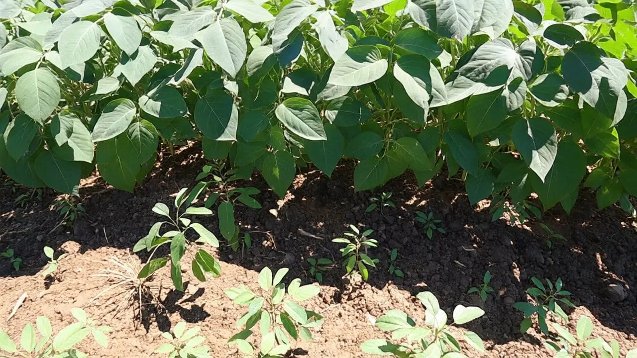
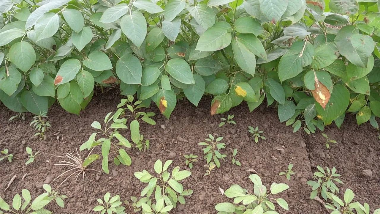
Generation Quality: Base vs Post-Trained

Side-by-side comparison on the same agricultural inputs:

Criterion	Base Cosmos Transfer 2.5	Post-Trained (Aigen)
Leaf morphology	Generic / incorrect species	Species-appropriate (trifoliate soybean)
Soil texture	Generic brown surface	Realistic dry tilled soil
Shadow consistency	Disconnected from plant geometry	Aligned with lighting direction
Weed diversity	Limited variation	Natural variation in species, size, placement
Depth control adherence	Weak	Strong — structure matches depth maps

Base Cosmos Transfer 2.5 Checkpoint

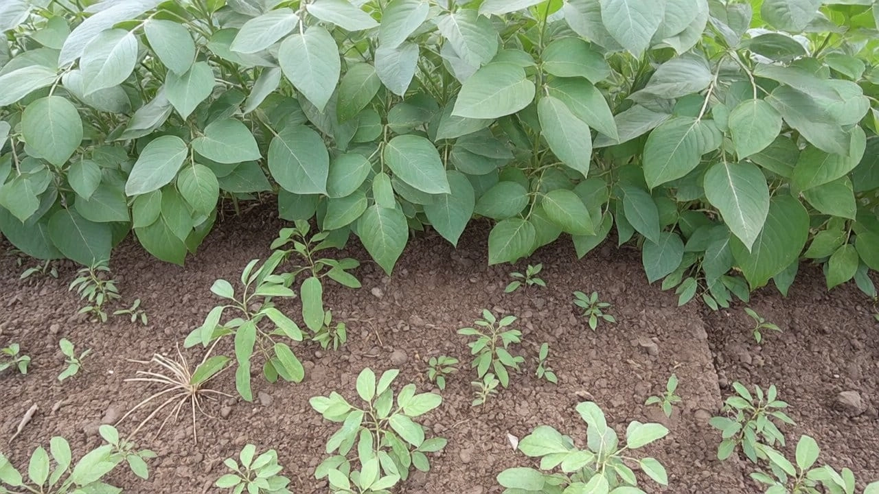Aigen's post-trained Cosmos Transfer 2.5

Downstream Impact

The post-trained model has been integrated into Aigen's perception model training pipeline:

Autonomous field weeding achieved using a perception model trained with only 1% real data, with the remainder generated synthetically using this pipeline.

This demonstrates that post-trained synthetic data is realistic enough to substitute for the majority of real-world data collection and human labeling.

Cross-Domain Generalization

The post-trained checkpoint was applied to crops outside the training distribution (e.g., fruit trees). Results are promising — the model produces reasonably realistic outputs for unseen crops, though not as consistently as for the soybean, cotton, and tomato fields seen during training.

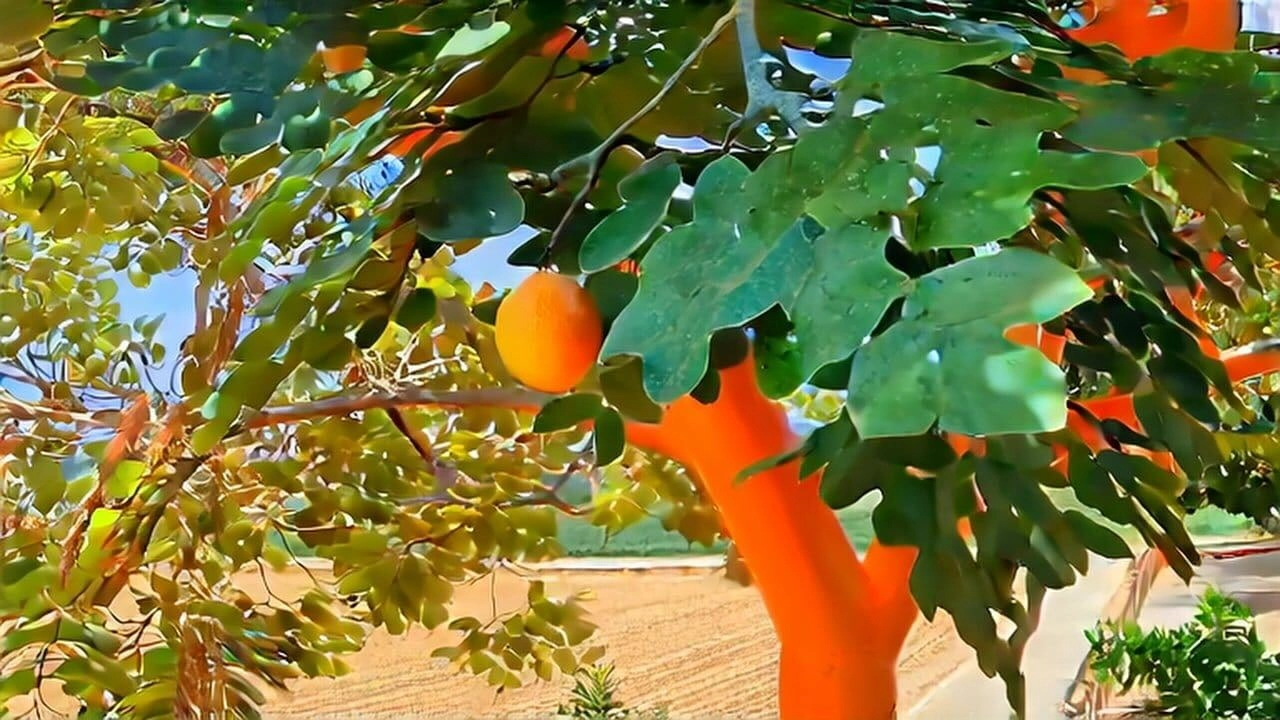Baseline sim2real

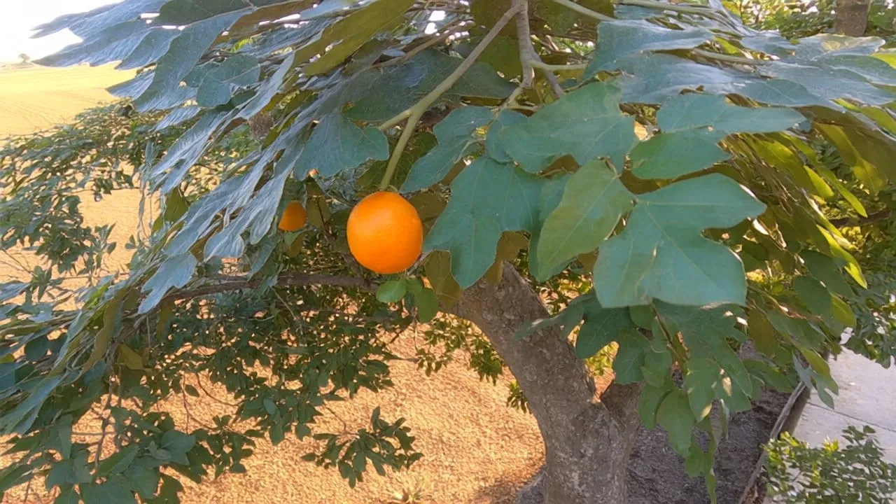Aigen post-trained sim2real

This suggests post-training efficiently activates the foundation model's latent understanding of natural scenes rather than overfitting to the training crops. For production-quality generation across a wider crop variety, a larger post-training run on more diverse data would be needed.

Disease Condition Synthesis

Prompt engineering enables diseased crop imagery without disease-specific training data. By describing visual symptoms (yellowing leaves, brown spots, wilting, lesions) in the text prompt, the model produces plausible disease presentations. This is particularly valuable because diseased crop data is rare and difficult to collect systematically in the real world.

Conclusion

Post-training Cosmos Transfer on agricultural fleet video is an effective approach to generating photorealistic synthetic data for precision agriculture robotics. Key findings:

Depth over edge for outdoor scenes with uncontrolled lighting — edge maps are corrupted by shadows and variable sunlight; depth is illumination-invariant
Train past loss plateau — visual quality continues improving after the loss curve flattens
Generalizes to unseen crops — post-training extends the foundation model's latent knowledge, not just overfits to training crops
Disease synthesis via prompting — disease data without disease-specific training examples
1% real data is sufficient for a production weeding system

Next steps

Expand crop diversity — post-train on a broader set of crops and field conditions to improve cross-domain generalization beyond soybean, cotton, and tomato.
Scale training iterations — longer training runs with larger datasets may further improve realism, especially for out-of-distribution crops.
Integrate video-level outputs — explore using generated video clips (rather than extracted frames) directly in temporal perception pipelines.
Benchmark against real data — systematically compare downstream perception metrics (mAP, IoU) across different real-to-synthetic data ratios to quantify the tradeoff.

Citation

@misc{cosmos_cookbook_sim2real_agriculture_2026,
  title={Sim2Real for Agriculture via Cosmos Transfer Post-Training},
  author={Author Names},
  organization={Aigen},
  year={2026},
  howpublished={\url{https://nvidia-cosmos.github.io/cosmos-cookbook/recipes/post_training/transfer2_5/singleview_domain_transfer/post_training.html}},
  note={NVIDIA Cosmos Cookbook}
}